Changing compatibility of localized spatial packets

Summary: A prescribed free-encounter functional separates reciprocal spatial deformation from free motion; the same local scalar dynamics can increase or decrease it for fully localized complex preparations, with its first change beginning beyond the leading scattering variation.

Compare both patterns using the same spatial rule

Use the local scalar Dirac equation

$$i\partial_t\Psi=D\Psi+g\sigma\beta\Psi, \quad D=-i\alpha\cdot\nabla, \quad \sigma=\Psi^\dagger\beta\Psi, \tag{1}$$

with its full complex source and reciprocal variation as in Dirac source linearization. The incoming field is a sum of two opposite complete kinetic chiralities, $\Psi=\Psi_u+\Psi_v$. Their individual scalar self-currents vanish, while their cross pattern supplies the entire scalar. The positive-frequency vertices retain its polarization, phase and spatial interference.

For a fixed comparison duration $T>0$, let $U(t)=e^{-iDt}$ and define

$$\boxed{\mathcal C_T[\psi]= \int_0^Tdt\int d^Dx\, \left[(U(t)\psi)^\dagger\beta U(t)\psi\right]^2.} \tag{2}$$

Both complete fields enter (2). A fixed target, a count of components, or an isotropic density replacement would define a different functional. It is nonnegative and uses exactly the scalar entering (1). With dimensionless positive norm and $\hbar=c=1$, $[\mathcal C_T]=\mathrm{length}^{1-D}$, so $g\mathcal C_T$ is dimensionless. It is not a measured interaction probability or a particle reaction rate.

The free propagation in (2) specifies a controlled encounter for the chosen preparation and duration. It permits reproducible comparisons of spatial patterns without declaring every overlap measure physically interchangeable. It is the spatially localized counterpart of the traveling-pulse compatibility comparison.

Remove the known free evolution before comparing outgoing patterns

Let $\Psi_g(t)$ solve the full nonlinear equation from $\psi_{\rm in}$. At time $T$ define

$$\boxed{\psi_{\rm out}^{I}=U(-T)\Psi_g(T).} \tag{3}$$

The same unitary inverse removes the free evolution of both chiral patterns. Compare

$$\Delta\mathcal C_T= \mathcal C_T[\psi_{\rm out}^{I}]-\mathcal C_T[\psi_{\rm in}]. \tag{4}$$

If $g=0$, (3) returns the incoming field exactly and (4) vanishes. The control retains every generated component; it does not project the outgoing field back into the incoming positive-frequency band or remove its spatial deformation. Individual chiral norms are reported separately.

Equation (3) is a mathematical comparison protocol. It does not assert that freely departing packets spontaneously refocus or encounter one another again. The sign of (4) says how the complete outgoing patterns perform in the specified subsequent free-encounter test. It is not a universal, protocol-independent definition of compatibility.

The first scattering variation preserves this functional

Use the positive spatial inner product and the complex gradient convention

$$\delta\mathcal C_T=2\operatorname{Re} \langle\nabla_*\mathcal C_T,\delta\psi\rangle. \tag{5}$$

Vary the local scalar before integrating. Its exact gradient is

$$\boxed{ \nabla_*\mathcal C_T[\psi] =2\int_0^Tdt\,U(-t) \left[\sigma(U(t)\psi)\,\beta U(t)\psi\right].} \tag{6}$$

The finite spatial regulator uses the orthogonal Galerkin projection of the displayed source and the same kinetic norm; no additional interaction coefficient appears.

Duhamel's formula for (1), at fixed $T$ and in a regime where the small-$g$ expansion is valid, gives

$$\boxed{\psi_{\rm out}^{I} =\psi_{\rm in}-\frac{ig}{2} \nabla_*\mathcal C_T[\psi_{\rm in}]+O(g^2).} \tag{7}$$

Consequently the first derivative of (4) at $g=0$ is

$$2\operatorname{Re}\left\langle \nabla_*\mathcal C_T,-\frac{i}{2}\nabla_*\mathcal C_T \right\rangle=0, \qquad \boxed{\Delta\mathcal C_T=O(g^2).} \tag{8}$$

The leading field deformation can therefore be nonzero while the leading change in this particular compatibility measure vanishes. Its later change depends on the evolving kinetic and source response. Equation (8) does not fix that change's sign or impose alignment.

Fully localized five-dimensional preparations

The axial spatial family reconstructs all five ordinary spatial directions while retaining both complete complex polarization vectors. It is a declared angular family of unbound fields, not a selected neutrino or another bound particle geometry.

Let $R_b(p,z_0,w_z,\xi)$ denote the unit-norm positive-frequency projection of the following raw field in chiral block $b$:

$$\phi_0^0(r)\,W\xi\, (\pi w_z^2)^{-1/4} \exp\left[-\frac{(z-z_0)^2}{2w_z^2}+ip(z-z_0)\right], \tag{9}$$

with radial scale $w=2$ and the normalized physical radial basis of the axial note. The projection uses the complete free spatial Dirac operator. Every $R_b$ is spatially localized and lies in its full positive free band. Its transverse profile is a Gaussian preparation, not a confining potential.

Set $\eta=0.6$, $\vartheta=0.7$, $b=(\cos\vartheta,e^{0.31i}\sin\vartheta)^T$, and let $S$ swap the two polarization coordinates. Prepare

$$\begin{aligned} u_0&=R_u(2,-4,2,e_1) +\eta e^{0.6i}R_u(2.35,-3,1.5,e_2),\\ v_0&=e^{i\varphi}R_v(-2,4,2,b) +\eta e^{-0.4i}R_v(-1.7,3,2.3,Sb),\\ \psi_{\rm in}&=u_0/\|u_0\|+v_0/\|v_0\|. \end{aligned} \tag{10}$$

Thus both full incoming patterns have positive norm one. The parameter $\varphi$ changes the phase of the main mode of the second pattern relative to its additional texture mode. It is not a global phase change of that entire pattern. The first pattern also has a nonconstant complex polarization texture; neither side is a fixed target.

Evolve (1) with the same $g=50$ and $T=10$ in both cases below. These are specified numerical units. Since $[g]=\mathrm{length}^{D-1}$, comparing this number with a coefficient in another spatial dimension would require its physical normalization; no common observed hierarchy coupling is inferred.

The complete nonlinear equation produces both signs at the same coupling. The effects are small. They show changing compatibility under the defined control, not attraction toward an automatically preferred orientation. The actual outgoing fields also differ from their free controls, with full positive-norm distances approximately $0.03223$ and $0.02698$.

A fixed-parameter phase scan

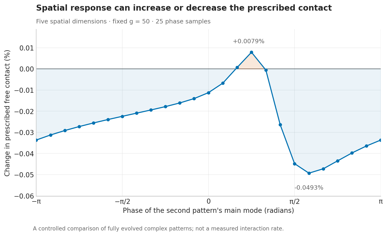
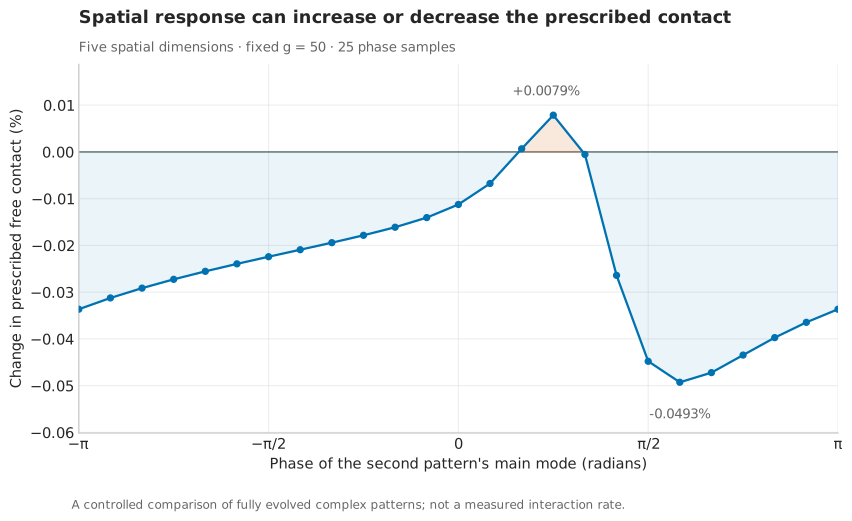
A scan of 25 phases from $-\pi$ to $\pi$, with the same preparation (10), norms and $g=50$, finds both signs. The sampled changes range from about $-0.0493\%$ to $+0.0079\%$. The connecting lines guide the eye; these are discrete preparations, not a fitted continuous law or a proof that the sampled extrema are the global extrema.

The recorded phase data contain each preparation, incoming and outgoing-control contact, and conserved-quantity errors. The vector figure and plotting code provide a reproducible display of those values. The scan uses radial cutoff 16 and 128 axial points; the more refined calculations above check the positive and negative examples at phases $0.7$ and $0$. Additional cutoff-40, 192-point checks of the sampled maximum at $\pi/4$ and minimum at $7\pi/12$ change their relative-contact values by less than $10^{-10}$. Those refinements are included in the recorded data; they do not locate a continuous global extremum.

Separate pattern change from redistribution of norm

For nonzero chiral norms $Q_u,Q_v$, define the same encounter with each complete pattern rescaled by its positive real norm:

$$\boxed{\mathcal S_T[\psi] =\mathcal C_T\left[\frac{\psi_u}{\sqrt{Q_u}} +\frac{\psi_v}{\sqrt{Q_v}}\right] =\frac{\mathcal C_T[\psi]}{Q_uQ_v}.} \tag{11}$$

The equality follows because each individual chiral scalar vanishes, free evolution preserves both chiral norms, and the cross scalar scales by $1/\sqrt{Q_uQ_v}$. Every relative phase and every spatial component is retained. This removes an amplitude product from the comparison; it does not replace the actual nonlinear evolution by renormalized dynamics.

For the two refined preparations in the table, both final chiral norms differ from one by less than $1.2\times10^{-8}$. Recomputing the comparison with (11) changes their reported $\Delta\mathcal C_T/ \mathcal C_T$ values by less than $6\times10^{-12}$ in absolute value. Both signs and their displayed sizes survive. The decrease is therefore not explained by a loss of the product of the two chiral norms.

More generally, start with equal norms $Q_u=Q_v=q>0$, and put $q_1=\partial_g Q_u|_{g=0}$. Conservation of their sum gives $Q_uQ_v=q^2-g^2q_1^2+O(g^3)$. If $\Delta\mathcal C_T=g^2c_2+O(g^3)$, then

$$\boxed{\frac{\Delta\mathcal S_T}{\mathcal S_{T,\rm in}} =g^2\left[\frac{c_2}{\mathcal C_{T,\rm in}} +\left(\frac{q_1}{q}\right)^2\right]+O(g^3).} \tag{12}$$

The direct coupling variations calculate $c_2$ and both norm variations from the complete field equation. The normalized comparison still uses the prescribed encounter protocol; it is not a universal definition of a measured coupling.

Predict the change before fitting any collisions

For preparation (10), the direct field variations give

$$\frac{\Delta\mathcal S_T}{\mathcal S_{T,\rm in}} =g^2 A_\varphi+O(g^3),\qquad A_0\simeq-4.761061\times10^{-8},\quad A_{0.7}\simeq+2.304888\times10^{-8}. \tag{13}$$

These coefficients come from differentiating the complete local equation at $g=0$, with both first and second spatial variations retained. They are not fitted to the nonlinear encounters. At phase $0.7$, raising the radial cutoff from 20 to 40 and the axial grid from 128 to 192 changes the coefficient by less than $6\times10^{-9}$ of its magnitude. The phase-zero cutoff-32 and cutoff-40 values agree more closely. The displayed digits describe this numerical model, not physical precision.

Full nonlinear evolution approaches those predictions:

As an independent perturbative control, also compute the encounters at $-g$ and average the two relative changes before dividing by $g^2$. This cancels the cubic contribution. At $|g|=25$ the two coefficients are $-4.757959\times10^{-8}$ and $+2.306713\times10^{-8}$; at $|g|=12.5$ they are $-4.760285\times10^{-8}$ and $+2.305344\times10^{-8}$. Their errors relative to (13) decrease by approximately four on halving $|g|$, as the remaining quadratic error in this quotient predicts. Changing the coefficient's sign here is a mathematical control, not an assignment of a physical interaction.

The recorded variation study contains five direct spatial refinements, ten nonlinear comparisons, both norm corrections, conserved-quantity errors and numerical source hashes. To reproduce a refined direct coefficient:

OPENBLAS_NUM_THREADS=1 OMP_NUM_THREADS=1 MKL_NUM_THREADS=1 \
python experiments/spatial_packet_variations.py \
  --radial-size 40 --axial-size 192 --phase .7

The nonlinear comparison uses axial_packet_benchmarks.py with --dimension 5 --radial-size 24 --axial-size 128 --texture .6 --polarization-angle .7 --phase .7 --coupling 12.5 --rtol 2e-12 --contact-order 128. Both programs write timestamped reports.

Verification and scope

axial_packet_benchmarks.py implements the exact preparation (10), complete nonlinear evolution and (2)–(4), with timestamped reports and optional full coefficient fields. For example:

OPENBLAS_NUM_THREADS=1 OMP_NUM_THREADS=1 MKL_NUM_THREADS=1 \
python experiments/axial_packet_benchmarks.py \
  --dimension 5 --radial-size 40 --axial-size 192 \
  --coupling 50 --rtol 2e-12 --texture .6 \
  --polarization-angle .7 --phase 0 --contact-order 128

Changing --phase to .7 gives the second preparation. --output-dir selects a directory for the timestamped numerical reports and optional coefficient fields.

The two signs survive radial cutoffs 16, 24, 32 and 40, axial refinement from 128 to 192 points, stricter adaptive integration and time quadrature from 64 to 128 nodes. The last quadrature change alters the reported relative changes by less than $10^{-14}$. Increasing the axial interval from $[-16,16]$ to $[-20,20]$ changes the two relative differences by less than $5\times10^{-11}$. The finite interval is a numerical regulator of localized ordinary spatial fields, not a physical compactification.

packet_compatibility_checks.py runs 26 checks. It independently integrates the free kinetic equation with an accumulated local scalar square, verifies the full complex derivative (6), and checks the first-order field map and quadratic compatibility change against complete nonlinear evolution. It also verifies canonical normalization and positive-frequency preparation of both textured incoming fields.

These calculations establish a conditional spatial response of the local scalar term. They do not supply bound-particle solutions, identify electric or weak channels, determine physical widths or derive observed coupling rates. The comparison complements those missing calculations; it does not replace them.

axial_packet_study.py repeats the specified preparation over a phase interval while keeping both norms, polarization vectors, widths, encounter duration and coupling fixed. Each case reports its own incoming and outgoing-control contact and conserved-quantity errors.

Time ordering of spatial compatibility derives the first nonzero contact coefficient from the Poisson bracket of the full source Hamiltonians at different encounter stages. Its complete complex variation distinguishes ordered feedback from the leading integrated overlap.